Data processing is commonly generated on software such as Matlab, where extensive spreadsheets are created as output to a variety of modeled systems or processes. In such fashion, a Simple Harmonic Movement can be coded in Matlab and the output behavior of the moving mass can be stored on a single column of numbers file that can later map the X, Y or Z position of the virtual sound source rendered through ViMiC.
As stated before, this method for Sonification can be considered a MBS, because the sound is not itself created by the data coming from spreadsheets, but rather the behavior that some arbitrary sound is following (in this case the position in virtual space) is created based on the data mapping. But it can also be considered a PM Sonification system, making the mapping of raw data into sound creation parameters available in a flexible structure.
The Sonification program is designed in such ways that the data files are read from a central hub and streamed in a bus-like thread. This data stream can then be used by any part of the program to control frequency of pure tones, gains, position in virtual space, and playback speeds.
The illustration of using Matlab as engine to produce for instance, Damped Simple Harmonic Movement (DSHM) data to later be used to sonify is just an example of the flexibility of the communication between Matlab and MAX/MSP. Further discussion can include the design of much more complex processes within Matlab with growing sophistication in regard to the connection with the Sonification engine. So, spatial related data sets can be conditioned on Matlab to be easily mapped into spatialized sound in MAX/MSP, through ViMiC, i.e. data such as global population density or economic displacements, that involve planet coordinates for instance.
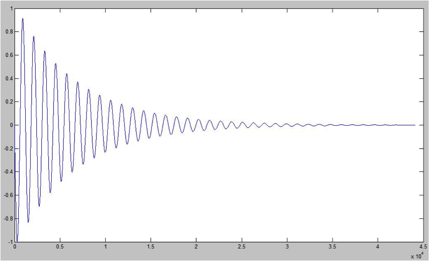
The next figure shows the output graph of a DSHM data output created on Matlab following notes from (Kemp, SHM, 2011). It plots the normalized amplitude of the movement with controlled spring constant, damping constant, mass, initial position and velocity.
Figure 11. DSHM picture, normalized to display values from -1 to 1 and over a period of 1 second, using 44100 data points.
Figure 11 shows that the output is composed of 44100 data points, that is equal to one second worth of sound (or control). This model then creates 44100 positions in a one-dimension vector on Matlab containing the amplitude of the movement at each sample. This vector is then saved as a spreadsheet that was later saved as a .csv file (more about this formatting comes later), and read on MAX/MSP.
It’s easy to see that this vector can be useful to control a variety of parameters on a Sonification or Spatialization model. This is just and illustrated example of the ideas on mind when I say mapping scientific or complex data into the system here presented.
…
Further on this chapter:
0. CONTENT
3.1 SPATIALIZATION USING SPATIAL DATA
